The War of the End of the World: The health puzzle posed by its survivors

The War of Canudos took place in Brazil in 1896 and 1897. Canudos was a settlement of several thousand deeply religious Christians, led by a man known as Antonio Conselheiro. They opposed the recent establishment of the Republic of Brazil, particularly the institution of income taxes and civil marriage; the former was considered government-sponsored theft and the latter a sacrilege. The republic had been declared in 1889 following a military coup that deposed Dom Pedro II, an emperor beloved by the common people and under whose rule slavery had recently been abolished.

Canudos was located in the Brazilian sertão, an inhospitable semi-arid region in the northeastern part of the country. The inhabitants of Canudos were the sertanejos. The term jagunço was used to refer to the males, especially the outlaws. Many of the sertanejos lived in semi-starvation, in poor sanitary conditions, and with very limited (if any) access to healthcare. Infant mortality was very high at the time. Those who reached adulthood were typically of small stature, and very thin; not lean, thin – often described as “skin and bones”.

Below is what a typical young jagunço would look like at the time of the War of Canudos. (Some authors differentiate between jagunços and cangaceiros based on small differences in cultural and dress traditions; e.g., the hat in the photo is typical of cangaceiros.) The jagunços tended to be the best fed among the sertanejos. They were also known as cold-blooded killers. The photo is a cropped version of the original one; the grizzly original is at the top of a recent blog post by Juan Pablo Dabove (). The blog post discusses Vargas Llosa’s historical fiction book based on the War of Canudos, the masterpiece titled “The War of the End of the World” ().

Jorge Mario Pedro Vargas Llosa, a Peruvian-Spanish writer and politician, was the recipient of the 2010 Nobel Prize in Literature; “The War of the End of the World” is considered one of his greatest literary achievements. Euclides da Cunha wrote the most famous non-fictional account on the War of Canudos, another masterpiece that has been called “Brazil’s greatest book”, titled “Rebellion in the Backlands” (). The Portughese title is “Os Sertões”. Vargas Llosa’s book is based on da Cunha’s.

Sergio Rezende’s movie, “Guerra de Canudos” (), is a superb dramatization of the War of Canudos. I watched this movie after reading Vargas Llosa’s and da Cunha’s books, and was struck by two things: (a) the outstanding performances, especially by José Wilker, Cláudia Abreu, Marieta Severo, and Paulo Betti; and (b) the striking resemblance of the latter (Betti) to Royce Gracie (), a very nice man whom I interviewed () for my book on compensatory adaptation (), and who is no stranger to Ultimate Fighting Championship and mixed martial arts fans ().

In a nutshell, the War of Canudos went more or less like this. There were four military campaigns against the settlement. The third was a major one, led by one of Brazil’s most accomplished military leaders at the time, Colonel Antônio Moreira César. The jagunços, resorting to guerrilla warfare, fought off the government troops in the first three. The fourth, led by General Arthur Oscar de Andrade Guimarães, saw the jagunços defeated in a war of attrition primarily due to lack of access to food and water, after heavy losses among government troops. At the end, nearly all of the surviving jagunços were executed, by knife – to their absolute horror, and the perverse pleasure of the executioners bent on revenge, as the victims believed that they would not go to heaven if their lives were ended by knife, even against their will.

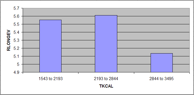
Ned, what is your point regarding health!?

After going through numerous sources, paper-based and online, academic and non-academic, I am convinced that a significant number of the survivors of the Canudos War lived to their 90s and beyond. This conclusion is based chiefly on comparisons of various dates, especially of interviews with survivors. No single source dedicated to this particular health-related aspect of the War of Canudos seems to exist. There is a video clip that shows some of the survivors (), speaking in Portuguese, with their ages shown in subtitles (“years”, in Portuguese, is “anos”). One of them, a man, is listed as being a supercentenarian.

In modern USA those who live to the age of 90 and beyond are outliers. Less than 2 percent of the population reach the age of 90 (). Most of them are women. My impression is that among the survivors of the War of Canudos, the 90+ percentage was at least 5 times higher; even with access to sanitation and healthcare in modern USA being much better at any age.

If my impression is correct, how can it be explained?

I think that some of the readers of this blog will be tempted to explain the high longevity based on calorie restriction. But the empirical evidence suggests that poor nutrition, in terms of micronutrients and macronutrients, is associated with increased mortality, not the other way around (, , ). Mortality due to poor nutrition is frequently from infectious diseases, in the young and the old. Degenerative diseases are widespread among the overnourished, not the well nourished, and kill mostly at later ages. It is not uncommon for infectious diseases to “mask” as degenerative diseases – e.g., viral diabetes ().

Often people point at hunter-gatherer populations and argue that they are healthy because of their low calorie intake. But mortality from infectious diseases among hunter-gatherers is very high, particularly in children. Others point to the absence of industrial foods engineered for overconsumption, which I think is definitely a factor in terms of degenerative diseases. Some say that a main factor is retention of lean body mass as one ages, referring mostly to muscle tissue, a hypothesis to which the case of the sertanejos poses a problem – what lean body mass!? And, on top of all of their problems, the sertanejos regularly faced long droughts, which may be why they typically had a “dry” look.

Yet others point to low stress. It is reasonable to think that stress is a mediating factor in the development of many modern diseases. Still, the sertanejos living in Canudos have had to endure quite a lot of stress, before and after the War of Canudos. In fact, the depictions of their lives at around the time of the War of Canudos suggest very stressful, miserable lives, prior to the conflict; which in part explains the early success of a religious settlement where life was marginally better.

By the way, the traditional Okinawans have also endured plenty of stress (), and they have had the highest longevity rates in recorded history. Food scarcity has frequently been combined with stress in their case, as with many other long-living groups. Causality is complex here, probably changing direction in different subsets of the data, but I have long suspected that the combination of stress and overnourishment is a particular unnatural one, to which humans are badly maladapted.

A main factor is almost always forgotten: the effective immune systems of those who have been subjected to starvation, poor sanitation, lack of healthcare, and other challenges – especially in childhood – and survived to adulthood. And here some counterintuitive things can happen. For example, someone may be very sickly early in life and barely survive childhood, and then become very resistant to infectious diseases later, thus appearing to be very healthy, to the surprise of relatives and friends who remember “that sickly child”. Immunocompetence is something that the body builds up in response to exposure.

As they say in northeastern Brazil, in characteristic drawl: “Ol’ sihtaneju ain’t die easy”.

The steep obesity increase in the USA in the 1980s: In a sense, it reflects a major success story

Obesity rates have increased in the USA over the years, but the steep increase starting around the 1980s is unusual. Wang and Beydoun do a good job at discussing this puzzling phenomenon (), and a blog post by Discover Magazine provides a graph (see below) that clear illustrates it ().

What is the reason for this?

You may be tempted to point at increases in calorie intake and/or changes in macronutrient composition, but neither can explain this sharp increase in obesity in the 1980s. The differences in calorie intake and macronutrient composition are simply not large enough to fully account for such a steep increase. And the data is actually full of oddities.

For example, an article by Austin and colleagues (which ironically blames calorie consumption for the obesity epidemic) suggests that obese men in a NHANES (2005–2006) sample consumed only 2.2 percent more calories per day on average than normal weight men in a NHANES I (1971–1975) sample ().

So, what could be the main reason for the steep increase in obesity prevalence since the 1980s?

The first clue comes from an interesting observation. If you age-adjust obesity trends (by controlling for age), you end up with a much less steep increase. The steep increase in the graph above is based on raw, unadjusted numbers. There is a higher prevalence of obesity among older people (no surprise here). And older people are people that have survived longer than younger people. (Don’t be too quick to say “duh” just yet.)

This age-obesity connection also reflects an interesting difference between humans living “in the wild” and those who do not, which becomes more striking when we compare hunter-gatherers with modern urbanites. Adult hunter-gatherers, unlike modern urbanites, do not gain weight as they age; they actually lose weight (, ).

Modern urbanites gain a significant amount of weight, usually as body fat, particularly after age 40. The table below, from an article by Flegal and colleagues, illustrates this pattern quite clearly (). Obesity prevalence tends to be highest between ages 40-59 in men; and this has been happening since the 1960s, with the exception of the most recent period listed (1999-2000).

In the 1999-2000 period obesity prevalence in men peaked in the 60-74 age range. Why? With progress in medicine, it is likely that more obese people in that age range survived (however miserably) in the 1999-2000 period. Obesity prevalence overall tends to be highest between ages 40-74 in women, which is a wider range than in men. Keep in mind that women tend to also live longer than men.

Because age seems to be associated with obesity prevalence among urbanites, it would be reasonable to look for a factor that significantly increased survival rates as one of the main reasons for the steep increase in the prevalence of obesity in the USA in the 1980s. If significantly more people were surviving beyond age 40 in the 1980s and beyond, this would help explain the steep increase in obesity prevalence. People don’t die immediately after they become obese; obesity is a “disease” that first and foremost impairs quality of life for many years before it kills.

Now look at the graph below, from an article by Armstrong and colleagues (). It shows a significant decrease in mortality from infectious diseases in the USA since 1900, reaching a minimum point between 1950 and 1960 (possibly 1955), and remaining low afterwards. (The spike in 1918 is due to the influenza pandemic.) At the same time, mortality from non-infectious diseases remains relatively stable over the same period, leading to a similar decrease in overall mortality.

When proper treatment options are not available, infectious diseases kill disproportionately at ages 15 and under (). Someone who was 15 years old in the USA in 1955 would have been 40 years old in 1980, if he or she survived. Had this person been obese, this would have been just in time to contribute to the steep increase in obesity trends in the USA. This increase would be cumulative; if this person were to live to the age of 70, he or she would be contributing to the obesity statistics up to 2010.

Americans are clearly eating more, particularly highly palatable industrialized foods whose calorie-to-nutrient ratio is high. Americans are also less physically active. But one of the fundamental reasons for the sharp increase in obesity rates in the USA since the early 1980s is that Americans have been surviving beyond age 40 in significantly greater numbers.

This is due to the success of modern medicine and public health initiatives in dealing with infectious diseases.

PS: It is important to point out that this post is not about the increase in American obesity in general over the years, but rather about the sharp increase in obesity since the early 1980s. A few alternative hypotheses have been proposed in the comments section, of which one seems to have been favored by various readers: a significant increase in consumption of linoleic acid (not to be confused with linolenic acid) since the early 1980s.

The lowest-mortality BMI: What is the role of nutrient intake from food?

In a previous post (), I discussed the frequently reported lowest-mortality body mass index (BMI), which is about 26. The empirical results reviewed in that post suggest that fat-free mass plays an important role in that context. Keep in mind that this "BMI=26 phenomenon" is often reported in studies of populations from developed countries, which are likely to be relatively sedentary. This is important for the point made in this post.

A lowest-mortality BMI of 26 is somehow at odds with the fact that many healthy and/or long-living populations have much lower BMIs. You can clearly see this in the distribution of BMIs among males in Kitava and Sweden shown in the graph below, from a study by Lindeberg and colleagues (). This distribution is shifted in such a way that would suggest a much lower BMI of lowest-mortality among the Kitavans, assuming a U-curve shape similar to that observed in studies of populations from developed countries ().

Another relevant example comes from the China Study II (see, e.g., ), which is based on data from 8000 adults. The average BMI in the China Study II dataset, with data from the 1980s, is approximately 21; for an average weight that is about 116 lbs. That BMI is relatively uniform across Chinese counties, including those with the lowest mortality rates. No county has an average BMI that is 26; not even close. This also supports the idea that Chinese people were, at least during that period, relatively thin.

Now take a look at the graph below, also based on the China Study II dataset, from a previous post (), relating total daily calorie intake with longevity. I should note that the relationship between total daily calorie intake and longevity depicted in this graph is not really statistically significant. Still, the highest longevity seems to be in the second tercile of total daily calorie intake.

Again, the average weight in the dataset is about 116 lbs. A conservative estimate of the number of calories needed to maintain this weight without any physical activity would be about 1740. Add about 700 calories to that, for a reasonable and healthy level of physical activity, and you get 2440 calories needed daily for weight maintenance. That is right in the middle of the second tercile, the one with the highest longevity.

What does this have to do with the lowest-mortality BMI of 26 from studies of samples from developed countries? Populations in these countries are likely to be relatively sedentary, at least on average, in which case a low BMI will be associated with a low total calorie intake. And a low total calorie intake will lead to a low intake of nutrients needed by the body to fight disease.

And don’t think you can fix this problem by consuming lots of vitamin and mineral pills. When I refer here to a higher or lower nutrient intake, I am not talking only about micronutrients, but also about macronutrients (fatty and amino acids) in amounts that are needed by your body. Moreover, important micronutrients, such as fat-soluble vitamins, cannot be properly absorbed without certain macronutrients, such as fat.

Industrial nutrient isolation for supplementation use has not been a very successful long-term strategy for health optimization (). On the other hand, this type of supplementation has indeed been found to have had modest-to-significant success in short-term interventions aimed at correcting acute health problems caused by severe nutritional deficiencies ().

So the "BMI=26 phenomenon" may be a reflection not of a direct effect of high muscularity on health, but of an indirect effect mediated by a high intake of needed nutrients among sedentary folks. This may be so even though the lowest mortality is for the combination of that BMI with a relatively small waist (), which suggests some level of muscularity, but not necessarily serious bodybuilder-level muscularity. High muscularity, of the serious bodybuilder type, is not very common; at least not enough to significantly sway results based on the analysis of large samples.

The combination of a BMI=26 with a relatively small waist is indicative of more muscle and less body fat. Having more muscle and less body fat has an advantage that is rarely discussed. It allows for a higher total calorie intake, and thus a higher nutrient intake, without an unhealthy increase in body fat. Muscle mass increases one's caloric requirement for weight maintenance, more so than body fat. Body fat also increases that caloric requirement, but it also acts like an organ, secreting a number of hormones into the bloodstream, and becoming pro-inflammatory in an unhealthy way above a certain level.

Clearly having a low body fat percentage is associated with lower incidence of degenerative diseases, but it will likely lead to a lower intake of nutrients relative to one’s needs unless other factors are present, e.g., being fairly muscular or physically active. Chronic low nutrient intake tends to get people closer to the afterlife like nothing else ().

In this sense, having a BMI=26 and being relatively sedentary (without being skinny-fat) has an effect that is similar to that of having a BMI=21 and being fairly physically active. Both would lead to consumption of more calories for weight maintenance, and thus more nutrients, as long as nutritious foods are eaten.

Maybe you should stop trying to be someone you are not

Many people struggle to lose body fat, and never quite make it to their optimal. Fewer people manage to do so successfully, and, as soon as they do, they want more. It is human nature. Often they will start trying to become someone they are not, or cannot be. That may lead to a lot of stress and frustration, and also health problems.

Some women have an idealized look in mind, and keep losing weight well beyond their ideal, down to anorexic levels. That leads to a number of health problems. For example, hormones approach starvation levels, causing fatigue and mood swings; susceptibility to infectious diseases increases significantly; and the low weight leads to osteopenia, which is a precursor to osteoporosis.

In men, often what happens is the opposite. Guys who are successful getting body fat to healthy levels next want to become very muscular, and fast. They have an idealized look in mind, and think they know how much they should weigh to get there. Sometimes they want to keep losing body fat and gaining muscle at the same time.

I frequently see men who already look very healthy, but who think that they should weigh more than they do. Since muscle gain is typically very slow, they start eating more and simply gain body fat. The reality is that people have different body frames, and their muscles are built slightly differently; these are things that influence body weight.

There are many other things that also influence body weight, such as the length of arms and legs, bone density, organ mass, as well as the amount of glycogen and water stored throughout the body. As a result, you can weigh a lot less than you think you should weigh, and look very good. The photo below (from MMAjunkie.com) is of Donald Cerrone, weighing in at 145 lbs. He is 6 ft (183 cm) tall.

Mr. Cerrone is a professional mixed martial arts (MMA) fighter from Texas; one of the best in professional MMA at the moment. Yes, he is a bit dehydrated on the photo above. But also keep in mind that his bone density is probably well above that of the average person, like that of most MMA fighters, which pushes his weight up.

A man can be 6 ft tall, weigh 145 lbs, and be very healthy and look very good. That may well be his ideal weight. A woman may be 5’5”, weigh 145 lbs, and also be very healthy and look very good. Figuring out the optimal is not easy, but trying to be someone you are not will probably be a losing battle.

Does strength exercise increase nitrogen balance?

This previous post looks at the amounts of protein needed to maintain a nitrogen balance of zero. It builds on data about individuals doing endurance exercise, which increases the estimates a bit. The post also examines the issue of what happens when more protein than is needed in consumed; including by people doing strength exercise.

What that post does not look into is whether strength exercise, performed at the anaerobic range, increases nitrogen balance. If it did, it may lead to a counterintuitive effect: strength exercise, when practiced at a certain level of intensity, might enable individuals in calorie deficit to retain their muscle, and lose primarily body fat. That is, strength exercise might push the body into burning more body fat and less muscle than it would normally do under calorie deficit conditions.

(Strength exercise combined with a small calorie deficit may be one of the best approaches for body fat loss in women. Photo source: complete-strength-training.com)

Under calorie deficit people normally lose both body fat and muscle to meet caloric needs. About 25 percent of lean body mass is lost in sedentary individuals, and 33 percent or more in individuals performing endurance exercise. I suspect that strength exercise has the potential to either bring this percentage down to zero, or to even lead to muscle gain if the calorie deficit is very small. One of the reasons is the data summarized on this post.

Two other reasons are related to what happens with children, and the variation in spontaneous hunger up-regulation in response to various types of exercise. The first reason can be summarized as this: it is very rare for children to be in negative nitrogen balance (Brooks et al., 2005); even when they are under some, not extreme, calorie deficit. It is rare for children to be in negative nitrogen balance even when their daily consumption of protein is below 0.5 g per kg of body weight.

This suggests that, when children are in calorie deficit, they tend to hold on to protein stores (which are critical for growth), and shift their energy consumption to fat more easily than adults. The reason is that developmental growth powerfully stimulates protein synthesis. This leads to a hormonal mix that causes the body to be in anabolic state, even when other forces (e.g., calorie deficit, low protein intake) are pushing it into a catabolic state. In a sense, the tissues of children are always hungry for their building blocks, and they do not let go of them very easily.

The second reason is an interesting variation in the patterns of spontaneous hunger up-regulation in various athletes. The increase in hunger is generally lower for strength than endurance activities. The spontaneous increase for bodybuilders is among the lowest. Since being in a catabolic state tends to have a strong effect on hunger, increasing it significantly, these patterns suggest that strength exercise may actually contribute to placing one in an anabolic state. The duration of this effect is approximately 48 h. Some increase in hunger is expected, because of the increased calorie expenditure during and after strength exercise, but that is counterbalanced somewhat by the start of an anabolic state.

What is going on, and what does this mean for you?

One way to understand what is happening here is to think in terms of compensatory adaptation. Strength exercise, if done properly, tells the body that it needs more muscle protein. Calorie deficit, as long as it is short-term, tells the body that food supply is limited. The body’s short-term response is to keep muscle as much as possible, and use body fat to the largest extent possible to supply the body’s energy needs.

If the right stimuli are supplied in a cyclical manner, no long-term adaptations (e.g., lowered metabolism) will be “perceived” as necessary by the body. Let us consider a 2-day cycle where one does strength exercise on the first day, and rests on the second. A surplus of protein and calories on the first day would lead to both muscle and body fat gain. A deficit on the second day would lead to body fat loss, but not to muscle loss, as long as the deficit is not too extreme. Since only body fat is being lost, more is lost on the second day than on the first.

In this way, one can gain muscle and lose body fat at the same time, which is what seems to have happened with the participants of the Ballor et al. (1996) study. Or, one can keep muscle (not gaining any) and lose more body fat, with a slightly higher calorie deficit. If the calorie deficit is too high, one will enter negative nitrogen balance and lose both muscle and body fat, as often happens with natural bodybuilders in the pre-tournament “cutting” phase.

In a sense, the increase in protein synthesis stimulated by strength exercise is analogous to, although much less strong than, the increase in protein synthesis stimulated by the growth process in children.

References

Ballor, D.L., Harvey-Berino, J.R., Ades, P.A., Cryan, J., & Calles-Escandon, J. (1996). Contrasting effects of resistance and aerobic training on body composition and metabolism after diet-induced weight loss. Metabolism, 45(2), 179-183.

Brooks, G.A., Fahey, T.D., & Baldwin, K.M. (2005). Exercise physiology: Human bioenergetics and its applications. Boston, MA: McGraw-Hill.

The China Study II: Does calorie restriction increase longevity?

The idea that calorie restriction extends human life comes largely from studies of other species. The most relevant of those studies have been conducted with primates, where it has been shown that primates that eat a restricted calorie diet live longer and healthier lives than those that are allowed to eat as much as they want.

There are two main problems with many of the animal studies of calorie restriction. One is that, as natural lifespan decreases, it becomes progressively easier to experimentally obtain major relative lifespan extensions. (That is, it seems much easier to double the lifespan of an organism whose natural lifespan is one day than an organism whose natural lifespan is 80 years.) The second, and main problem in my mind, is that the studies often compare obese with lean animals.

Obesity clearly reduces lifespan in humans, but that is a different claim than the one that calorie restriction increases lifespan. It has often been claimed that Asian countries and regions where calorie intake is reduced display increased lifespan. And this may well be true, but the question remains as to whether this is due to calorie restriction increasing lifespan, or because the rates of obesity are much lower in countries and regions where calorie intake is reduced.

So, what can the China Study II data tell us about the hypothesis that calorie restriction increases longevity?

As it turns out, we can conduct a preliminary test of this hypothesis based on a key assumption. Let us say we compared two populations (e.g., counties in China), based on the following ratio: number of deaths at or after age 70 divided by number deaths before age 70. Let us call this the “ratio of longevity” of a population, or RLONGEV. The assumption is that the population with the highest RLONGEV would be the population with the highest longevity of the two. The reason is that, as longevity goes up, one would expect to see a shift in death patterns, with progressively more people dying old and fewer people dying young.

The 1989 China Study II dataset has two variables that we can use to estimate RLONGEV. They are coded as M005 and M006, and refer to the mortality rates from 35 to 69 and 70 to 79 years of age, respectively. Unfortunately there is no variable for mortality after 79 years of age, which limits the scope of our results somewhat. (This does not totally invalidate the results because we are using a ratio as our measure of longevity, not the absolute number of deaths from 70 to 79 years of age.) Take a look at these two previous China Study II posts (here, and here) for other notes, most of which apply here as well. The notes are at the end of the posts.

All of the results reported here are from analyses conducted using WarpPLS. Below is a model with coefficients of association; it is a simple model, since the hypothesis that we are testing is also simple. (Click on it to enlarge. Use the "CRTL" and "+" keys to zoom in, and CRTL" and "-" to zoom out.) The arrows explore associations between variables, which are shown within ovals. The meaning of each variable is the following: TKCAL = total calorie intake per day; RLONGEV = ratio of longevity; SexM1F2 = sex, with 1 assigned to males and 2 to females.

As one would expect, being female is associated with increased longevity, but the association is just shy of being statistically significant in this dataset (beta=0.14; P=0.07). The association between total calorie intake and longevity is trivial, and statistically indistinguishable from zero (beta=-0.04; P=0.39). Moreover, even though this very weak association is overall negative (or inverse), the sign of the association here does not fully reflect the shape of the association. The shape is that of an inverted J-curve; a.k.a. U-curve. When we split the data into total calorie intake terciles we get a better picture:

The second tercile, which refers to a total daily calorie intake of 2193 to 2844 calories, is the one associated with the highest longevity. The first tercile (with the lowest range of calories) is associated with a higher longevity than the third tercile (with the highest range of calories). These results need to be viewed in context. The average weight in this dataset was about 116 lbs. A conservative estimate of the number of calories needed to maintain this weight without any physical activity would be about 1740. Add about 700 calories to that, for a reasonable and healthy level of physical activity, and you get 2440 calories needed daily for weight maintenance. That is right in the middle of the second tercile.

In simple terms, the China Study II data seems to suggest that those who eat well, but not too much, live the longest. Those who eat little have slightly lower longevity. Those who eat too much seem to have the lowest longevity, perhaps because of the negative effects of excessive body fat.

Because these trends are all very weak from a statistical standpoint, we have to take them with caution. What we can say with more confidence is that the China Study II data does not seem to support the hypothesis that calorie restriction increases longevity.

Reference

Kock, N. (2010). WarpPLS 1.0 User Manual. Laredo, Texas: ScriptWarp Systems.

Notes

- The path coefficients (indicated as beta coefficients) reflect the strength of the relationships; they are a bit like standard univariate (or Pearson) correlation coefficients, except that they take into consideration multivariate relationships (they control for competing effects on each variable). Whenever nonlinear relationships were modeled, the path coefficients were automatically corrected by the software to account for nonlinearity.

- Only two data points per county were used (for males and females). This increased the sample size of the dataset without artificially reducing variance, which is desirable since the dataset is relatively small (each county, not individual, is a separate data point is this dataset). This also allowed for the test of commonsense assumptions (e.g., the protective effects of being female), which is always a good idea in a multivariate analyses because violation of commonsense assumptions may suggest data collection or analysis error. On the other hand, it required the inclusion of a sex variable as a control variable in the analysis, which is no big deal.

- Mortality from schistosomiasis infection (MSCHIST) does not confound the results presented here. Only counties where no deaths from schistosomiasis infection were reported have been included in this analysis. The reason for this is that mortality from schistosomiasis infection can severely distort the results in the age ranges considered here. On the other hand, removal of counties with deaths from schistosomiasis infection reduced the sample size, and thus decreased the statistical power of the analysis.